Notes on Statistical Rethinking: Chapters 1-3

Chapter 1

The Problem with Deductive Falsification

Many people believe that the best way to do science, the proper objective of statistical inference, is to test null hypotheses. This way of thinking was popularized by Karl Popper, who argued that we can better deepen our understanding of the world by developing hypotheses that are falsifiable. However, deductive falsification is impossible in the vast majority of contexts.

The problem lies here: Many process models, explanations as to why a hypothesis is true, correspond to the same hypothesis. A traditional approach is then to use a statistical model to validate the explanation. But a single statistical model can validate explanations that correspond to different hypotheses.

An example follows. Since the 1960s, evolutionary biologists have been interested in the idea that evolutionary changes in gene frequency are not caused by natural selection, but by mutation and drift. This leads to the two hypotheses in the diagram below.

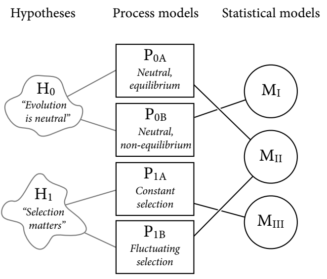
For each hypothesis there are potentially hundreds of possible process models. In the case of the null hypothesis H₀, researchers proposed P_0A and P_0B, which describe whether population size and structure have been stable for long enough for the distribution of alleles in a genetic sequence to reach a stable state.

For the hypothesis that evolutionary changes are caused by natural selection, again there are many possible process models. The diagram shows two; a model in which selection favours certain alleles, and another in which selection fluctuates through time, favouring different alleles.

M_II refers to a statistical model that can capture the expected frequency distribution of a quantity - a histogram. Process model P_0A would predict that alleles follow a power law distribution. However, P_1B would also entail that the distribution of alleles follows a power law. In this case, a statistical test seems to validate both the hypothesis that evolutionary changes in gene frequency are caused by natural selection, and the exact opposite.

Developing Better Hypotheses

One response to the above may be: “Why not develop more precise hypotheses?”. Consider the hypothesis “All swans are white.”

1. Imagine finding a swan that is a shade of grey. Is the swan white? This may be easy enough to debate, but in many fields the definition of the concept being measured is as much in question as its existence.
2. Most interesting hypotheses are continuous: “80% of swans are white.” This calls for a method that describes the colour distribution as accurately as possible, rather than something to falsify.

So, what next?

A Better Set of Tools

Statistical Rethinking proposes four main tools to design inquiry, extract information, make predictions, and argue the case for some causal explanation of a phenomenon. These are:

Bayesian Data Analysis

This process involves counting the number of ways you could get a set of observations. If an explanation can cause the data to arise in more ways, that explanation is more plausible. It turns out that if you have an idea of prior plausibility, you can use new information to update plausibility iteratively using Bayes’ Theorem.

Model Comparison

Models can produce predictions. You should prefer models that produce better predictions. This may imply having some understanding of the future, but there are tools you can use without owning a crystal ball: Cross-validation and information criteria.

There is a trade-off when building predictive models between optimization and generalizability. A model, retrofit on past data, can notice extremely complex patterns. Applying that model to make predictions on new data can lead to poor predictions, because the model was overfit to the unique circumstances under which the first dataset originated. A complex model can lack generalizability to new data.

The tools here combat overfitting, allowing models to generalize better.

Multilevel Models

While cross-validation and information criteria identify the risk of overfitting, multilevel models help us do something about it.

Observations are often clustered in ways that are not foreseen (for example, by location or year). Single-level models lack interpretability in the face of clustered observations.

1. If observations are sampled repeatedly for the same dimension (individual, location, time, etc.) single-level models can be misleading.
2. When some observations are sampled more frequently for one dimension, single-level models are again misleading.
3. If the research question requires an explanation of variation across different dimensions, single-level models are less interpretable than multilevel models.
4. Pre-averaging data across dimensions can remove variation, which removes important nuances in the model. Multilevel models preserve these nuances.

Graphical Causal Models

Wind causes tree branches to sway, tree branches do not cause wind to blow. A statistical model would be awesome at finding this association, but it would be absolutely terrible at describing what caused what.

To make matters worse, it turns out that causally incorrect models can make better predictions than causally correct models. This is because confounded relationships, where two variables X and Y appear to be correlated but in reality both are affected by an unobserved Z variable, are still real relationships. Observing swaying branches really would predict wind.

Rather than relying on models alone, a complete picture requires background understanding of the question - and a reasonable causative mechanism to explain the plausibility of the data.

This can be done with graphical causal models, the simplest version of which is a directed acyclic graph (DAG).

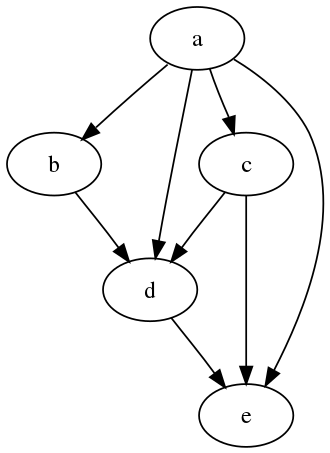
The creation of such graphs requires the use of information outside the data. While this sounds inherently unscientific, no model can accept data alone and give a reliable representation of causal mechanisms. Developing an understanding of reality is an iterative process of developing theories, judging the plausibility of each theory given the observations, and continuing to dig in the direction most likely to lead to truth.

Chapter 2

Small Worlds and Large Worlds

There is a contrast between the small world of a model and the large world of reality. The small world should provide the best possible representation of the large world, given that it cannot incorporate all of its information. This chapter focuses on the small world.

Bayesian Inference

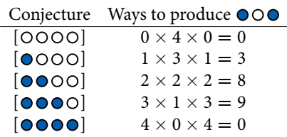
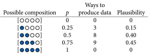
Bayesian models have a reasonable claim to being the optimal way of representing a large world with a small world, assuming the small world accurately descibes the large world. A Bayesian model uses Bayesian inference, which simply counts and compares possibilities. Consider a bag with four marbles in two colours, blue and white. There are 5 possible sequences:

Imagine you then pulled three marbles from the bag, in the order [B,W,B]. There is an explicit number of ways for this observation to occur, given each of the 5 possible sequences:

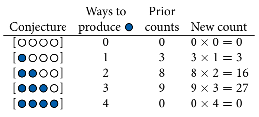
It turns out that, if you know the “prior” number of ways to produce [B,W,B], you can use this information to update on a 4th pick by multiplying the prior by the number of ways of producing the 4th pick. The example below shows the 4th pick as [B].

This is formalized below, where ∝ means “as a proportion of”:

You then need to standardize the number of ways into a probability, such that the total = 1.

Building a Model

The book gives the example of trying to work out how much of the Earth’s surface is covered by water with a simple experiment. You are given a hand-sized globe representing Earth. You toss it into the air and count the times your index finger lands on water (W) or land (L).

In this case:

1. The true proportion of water covering the globe is p.
2. A single toss has a probability p of touching water, and 1-p of touching land.
3. Each toss is independent of the others.

As you gain more information about the likelihood of W or L, you can update the proportion of water p as per the graphs below. The final plausibility value of p is an abbreviation of the iterative learning process.

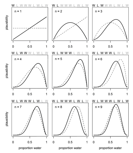
On the first toss the index finger landed on water. By the lights of the model, there is approximately 0% chance of a world with no water, and a high chance of the world being completely covered in water. On the second toss the index finger tounches land. There is approximately 0% chance of a world covered in either water or land, and the most plausible proportion p is 50/50. As the globe is tossed repeatedly, the most plausible p converges to its true value.

This is a simple Bayesian small world model. It learns well, provided that it accurately describes the large world. However, a model’s certainty is no guarantee of a good model, since it is confined to the information contained within the small world.

Components of the Model

There are three parts to a Bayesian model, all of which have a parallel in probability theory:

1. The number of ways each conjecture could produce an observation
2. The accumulated number of ways each conjecture could produce the entire data
3. The initial plausibility of each conjectured cause of the data

Since we are translating these parts to probability theory, we need to play by its rules.

Variables

Simply the symbols used to capture things we want to infer. In the example above, p is the proportion of water, and W/L are the counts of water and land respectively. Unobserved variables are usually called parameters. p is technically unobserved, but can be inferred from other variables.

Definitions

For each observed variable, we must define the number of ways the observation could have arisen. For each unobserved variable, we need to define the prior plausibility of each value it could take.

In this case, you can define the plausiblity of any combination of W/L for a specific value of p. Since there are only two events (W/L), each toss is independent, and the probability of W is the same each time, the analogy in probability theory is the binomial distribution.

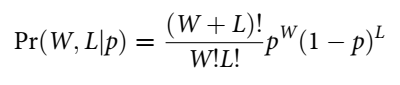
Read as: “The counts of W and L are distributed binomially, with probability p of water on each toss.”

Unobserved variables are typically called parameters. For each parameter, you must provide a distribution of prior probability (its prior). Without a strong intuition of prior, you can try different priors.

Resulting Model

W ~ Binomial(N, p) where N = W + L

p ~ Uniform(0, 1) such that p is a flat prior over all possible values from 0 to 1.

Making the Model Go

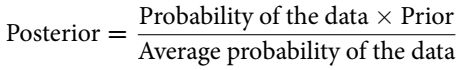
A Bayesian model can update prior distributions to their logical end based on new data, called the posterior distribution. The posterior is the left-hand side of the equation in Bayes’ theorem.

Motors

Since most interesting models in contemporary science cannot be conditioned formally in the same way as the example above, various techniques are required to approximate the maths that follows from Bayes’ theorem. Statistical Rethinking introduces three:

Grid Approximation

While parameters are continuous, you can get a good idea of the posterior distribution by testing different discrete values for each parameter. For complex models this is very computationally expensive, since the number of calculations scales quadratically for each new parameter.

Quadratic Approximation

Under regular conditions, the peak of a posterior distribution will be almost Gaussian or “normal” - the familiar bell curve distribution. Therefore, the entire posterior distribution can be approximated by a Gaussian distribution. This is useful since a Gaussian distribution can be completely described by the location of the centre (mean) and spread (variance).

There are optimization algorithms to find the peak of the distribution. When you calculate the plausibility of different sets of parameter values, you can calculate the slope corresponding to that plausibility on the posterior distribution by taking the derivative. Since you assume the distribution to be Gaussian and know the slope, you have an understanding of possible values that will take you up or down the slope to reach the peak. When you find the peak, understanding the curvature around the peak should give a good approximation of the entire posterior distribution.

Quadratic approximation often requires larger sample sizes, and can even remain inaccurate at thousands of samples. In that case, you may need to use another approximation.

Markov Chain Monte Carlo (MCMC)

Instead of approximating the posterior distribution directly, you can also draw samples from the posterior. This results in a collection of parameter values and their frequencies, which correspond directly to posterior plausibilities. This avoids having to model the posterior distribution entirely, making it possible to estimate very large models with far less compute.

Chapter 3

Bayes’ theorem is often introduced with an example in the following form:

• A test correctly detects vampirism 95% of the time, but gives a false positive 1% of the time.
• The population of vampires in the population is 0.01%.
• What is the probability of a person being a vampire, given that they tested positive?

This can be worked out with Bayes’ theorem.

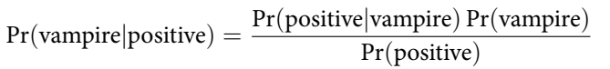
Where:

This gives a probability of 8.7%, which can seem unintuitive. However, if you frame the problem differently it becomes more clear.

• In a population of 100,000 people, 100 are vampires.
• Of the 100 vampires, 95 will test positive for vampirism.
• Of the 99,900 mortals, 999 will test positive for vampirism.

Thus, 8.7% of positive tests come from actual vampires. This way of approaching the problem relies on sampling counts, and is known as the frequency format or natural frequencies.

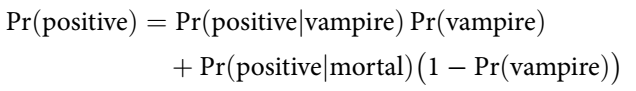
Sampling from a Grid-Approximate Posterior

When you have a posterior distribution, you can generate samples from it. The image below shows a sample of 10,000 tosses from the previous globe tossing example:

The more samples you generate, the closer to the ideal posterior distribution you get.

Sampling to summarize

With a posterior distribution in hand, you are now tasked with summarizing and interpreting the posterior distribution. The questions you may ask can be usefully sorted into the following three categories:

Intervals of defined boundaries

Such as “What is the posterior probability that the proportion of water is less than 0.5?”.

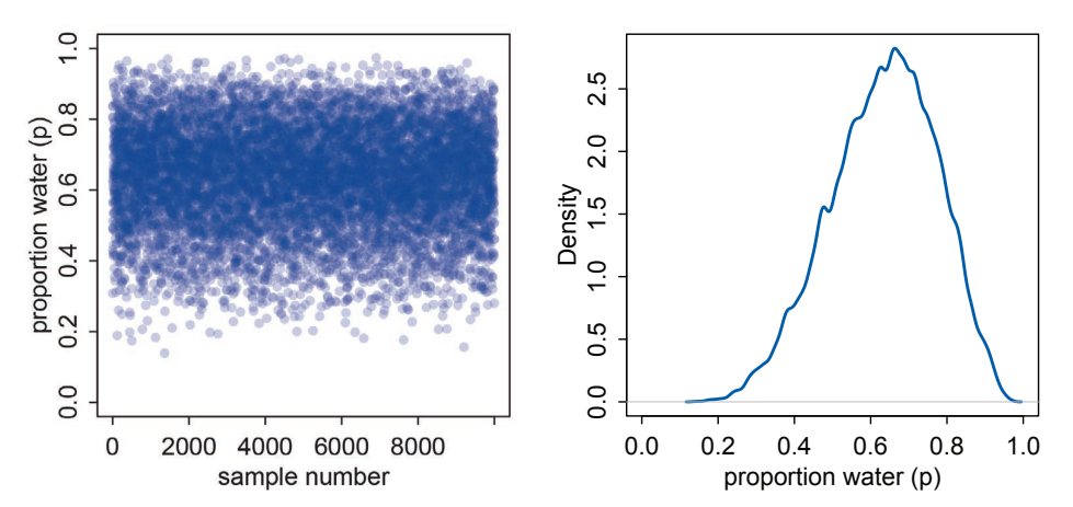
Intervals of defined mass

Otherwise known as confidence interval, or a credible interval when dealing with posterior distributions. The book uses the term compatibility interval to avoid the unwarranted connotations associated with the terms “confidence” and “credibility”. In the image below, the top row shows intervals of defined boundaries while the bottom row shows intervals of defined mass.

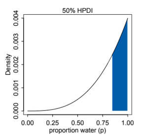
You may notice that are infinitely many compatibility intervals with the same mass, depending on where you place the interval. The Highest Posterior Density Interval (HPDI) is the narrowest interval with a specified proability mass. The following image shows the 50% HDPI for 3 globe tosses that resulted in [W,W,W].

Point estimates

Giving a single value to encapsulate a distribution is hardly ever necessary and often harmful. However, there are some questions you may want to ask of the distribution that could be useful.

One is the most plausible parameter, or the maximum a posteriori (MAP). You could also ask for the mean or median of the distribution. If you try to minimize the absolute loss between the real p and the one of the mean, median or mode, the median has the lowest loss (proof available in an endnote in the book). Minimizing quadratic loss (d-p)² leads to the mean. The loss function you choose to use depends on the question you are trying to answer.

Sampling to Simulate Prediction

A model can give predictions. Simulating observations can check the robustness of a model and its predictions.

In the globe tossing problem, given a value for p and a number of tosses, the binomial distribution implies a probability for each result. In the case of p=0.7 and n=2, the implied probability for 0, 1, and 2 water (W) results is [0.09, 0.42, 0.49] repectively. This can be used to create dummy data, which can be used alongside samples from the posterior distribution to check validity.

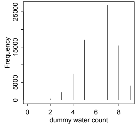
Model Checking

Checking model is an assessment of why a model is wrong. All models are wrong to some extent, but you must ensure the model is still fit for purpose.

One assumption of the globe tossing example is that each toss is independent of others. Looking at patterns over 9 tosses, the assumption is called into question.

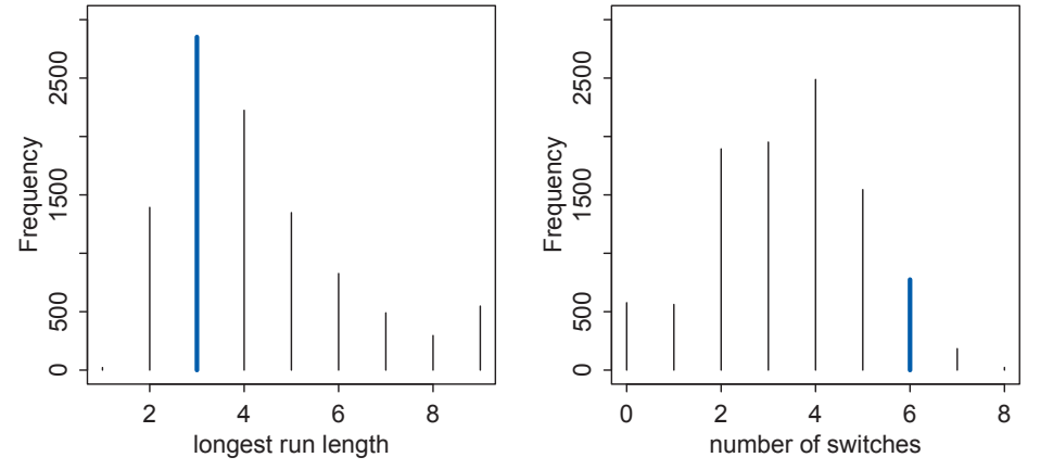
In this case, the number of times each subsequent toss switched between W/L is inconsistent with the expected posterior distribution. This implies that each toss is influenced to some degree by the previous toss, resulting in a posterior distribution that eventually converges to the true p, but would take longer to do so.